
Transcription of the manuscript Local Moves, Global Clusters (October 2026), including the proofs, appendix and 27 illustrations. References to gallery.html, videos and the reproduction folder describe the original manuscript’s supplement; this site’s interactive experiment and its code are available in the Numerical experiments section.
Abstract
We study finite-particle ascent and descent algorithms for symmetric interaction energies on a finite graph. The graph prescribes admissible one-particle moves; the interaction kernel need not be supported on its edges. For spherical embeddings whose convex-hull edges are all admissible, we prove that every terminal ascent configuration is a single cluster when the interaction parameter is sufficiently small. The bound is explicit, uniform over initial configurations, and stable under arbitrary small symmetric perturbations of the exponent. This framework contains products of cycles, hypercubes, inscribed polyhedral graphs and Hamiltonian graphs with a suitable kernel. A globally steepest implementation also satisfies an explicit bound on the number of accepted moves.
For trees with an exponential graph-distance kernel, we obtain an exact threshold for concentration from every initial configuration. Two counterexamples show why neither connectedness nor positive attraction alone suffices. For descent, we prove neighboring-occupation rigidity, spectral discrepancy estimates, a large-parameter asymptotic formula and quantitative pair-separation bounds. The original torus-specific Fourier and smooth-profile arguments are developed in full, with coordinate conventions made explicit. The exposition is intended for researchers and motivated students: every main claim is proved, while numerical experiments and animations illustrate rather than replace the mathematics. The link to self-attention is an energetic modeling connection, not a claim about the training or performance of a general Transformer.
How to read these notes
The main geometric route is Sections 2 to 4. Section 5 places the discrete torus inside that framework; Section 6 provides a second, intrinsically graph-theoretic route. The obstruction examples in Section 7 are part of the theory, not exceptions to be hidden. Readers interested in dispersion can proceed to Sections 8 and 9. The experiments and computational conventions appear in Sections 10 and 11. Section A records the complete smooth perturbation and one-dimensional profile arguments behind the torus proof.
Prerequisites are finite graph theory, elementary convex geometry, linear algebra, Taylor’s theorem, Fourier series on a finite abelian group, and the contraction mapping theorem. No transport geometry is used. All graphs are finite, simple and undirected. All numerical trajectories count accepted moves, not physical time or neural-network depth.
Reading the visual companion
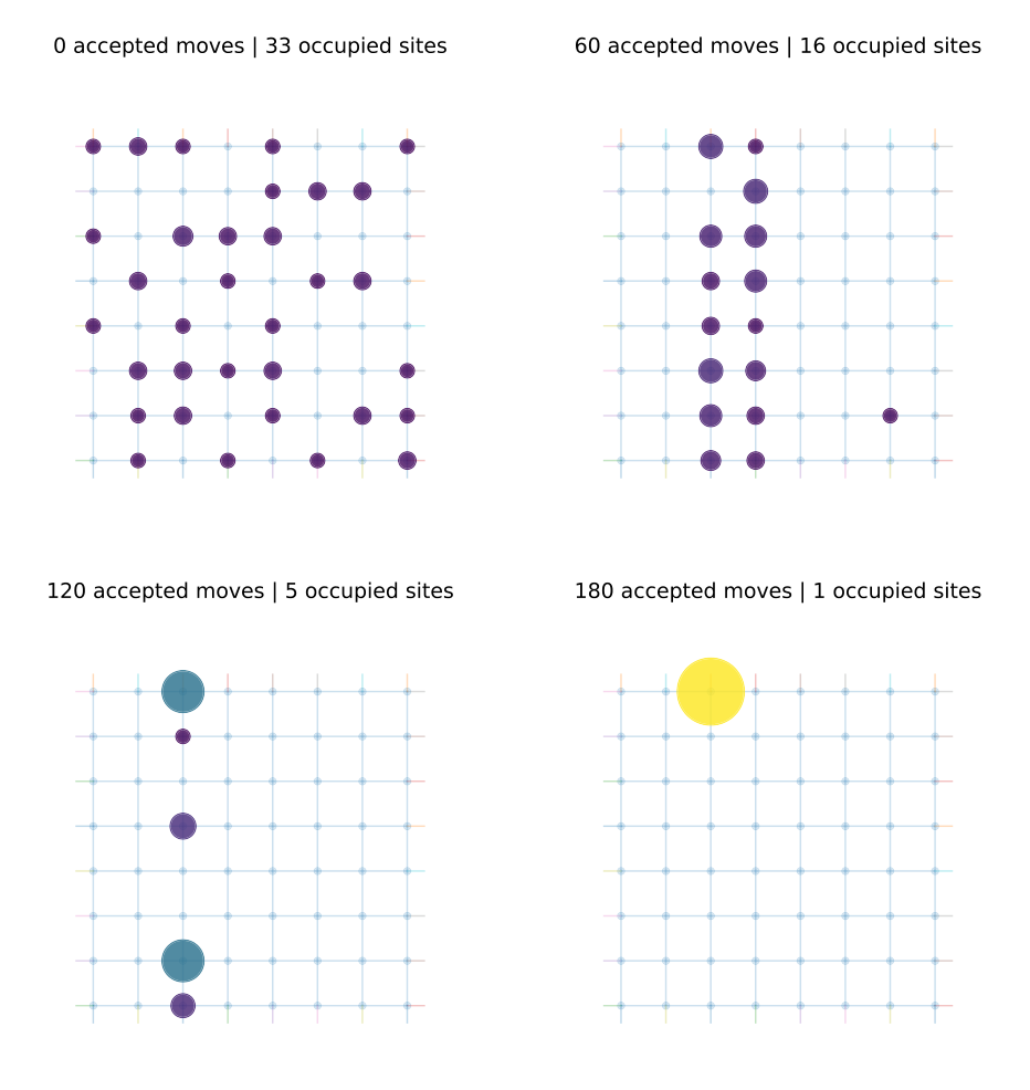
Bubble area encodes particle occupation; the colormap also records the number of particles at a site. Edges describe allowable moves, not all interactions. A three-dimensional drawing may be a projection of the actual embedding used in the kernel. Every such distinction is stated in the relevant caption. Static figures are embedded in this PDF. The five MP4 files and the offline HTML reader are supplied separately because embedded video is not reliably supported by PDF readers.
Notation at a glance
- \(G=(X,\mathcal E),\quad M=|X|\)
- The move graph and its number of vertices.
- \(p\sim q\)
- An allowed one-particle move along an undirected edge.
- \(n\)
- Number of particles; always an integer, and fixed in the theorems.
- \(c\in\mathcal C_n\)
- Occupation field: \(c(x)\in\{0,1,2,\ldots\}\) and \(\sum_xc(x)=n\).
- \(K,\quad V_c=Kc\)
- Symmetric interaction matrix and its induced potential.
- \(E_K(c)=c^\top Kc\)
- Total interaction energy, including self-interactions.
- \(\mathcal D_{p,q}E_K(c)\)
- Exact change when one particle moves from \(p\) to \(q\).
- \(v_x\in\mathbb R^m,\quad |v_x|=R\)
- Spherical embedding used in the geometric theorem.
- \(P=\operatorname{conv}\{v_x\},\quad\mathcal E_P\)
- Its convex hull and its set of edges.
- \(a_{xy}=\tfrac12|v_x-v_y|^2\)
- Squared chordal dissimilarity, not shortest-path distance.
- \(A,\delta,\gamma\)
- Respectively \(\max_{x,y}a_{xy}\), \(\min_{pq\in\mathcal E_P}a_{pq}\), and \(\min_{x\ne y}a_{xy}\).
- \(\overline K_\beta(x,y)=e^{-\beta a_{xy}}\)
- A normalized form of the exponential dot-product kernel.
- \(d_G,\quad D=\operatorname{diam}G\)
- Shortest-path distance and graph diameter.
- \(\mathcal H=\mathbf1^\perp,\quad\lambda_H\)
- The subspace of zero-sum vectors and the coercivity constant of \(K\) restricted to \(\mathcal H\).
- \(T\)
- Number of accepted moves before termination.
The three integers \(M,n,m\) have different meanings: number of sites, number of particles, and Euclidean embedding dimension. In the torus example, \(M=N^d\) whereas the convenient spherical embedding has dimension \(m=2d\). A graph may be drawn in two or three dimensions even when its kernel is defined using higher-dimensional vectors.
1 Why study local particle moves?
1.1 A simple experiment with a nontrivial outcome
Place \(n\) particles at vertices of a graph. Each particle sees the entire configuration through a similarity kernel, but can move only to a neighboring vertex. Accept a move when it increases the total similarity. The energy then increases and, because the state space is finite, the procedure eventually stops. None of this says that the particles have formed one cluster. A configuration may be globally suboptimal yet offer no improving one-step move.
This elementary distinction is the subject of these notes. We are not trying merely to identify a maximizer of an energy. We want to determine when the local geometry of the allowed moves forces an algorithm to find one, independently of its initial configuration and independently of the order of improving moves. Reversing the acceptance rule gives a repulsive algorithm, for which the appropriate questions concern dispersion, occupation differences and exclusion of excessively close pairs.
Animation 1. torus_ascent.mp4. The offline companion gallery.html provides playback and a state-by-state slider.
1.2 The attention connection: what is shared, and what is not
The attention operation introduced in the Transformer architecture assigns weights according to similarities between query and key vectors. In its scaled dot-product form, the weight from token \(i\) to token \(j\) is
where \(w_{j}\) denotes a value vector and \(d_{k}\) the key dimension [1]. Query, key and value maps are generally learned, possibly different, and layer-dependent. We will not retain all of that structure. Instead, we isolate the effect of a symmetric exponential similarity.
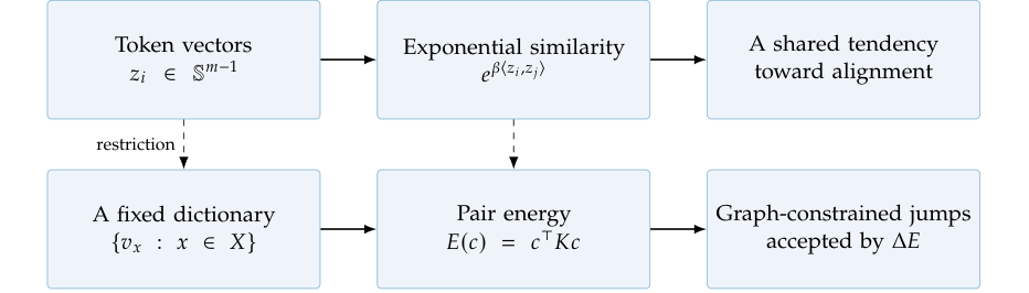
In particle descriptions of simplified self-attention, a token is represented by a point whose motion depends on the other points. This viewpoint is developed by Geshkovski, Letrouit, Polyanskiy and Rigollet [2, 3]. For unit vectors, the exponential similarity \(e^{\beta \langle z_{i},z_{j}\rangle}\) favors alignment. Geshkovski, Koubbi, Polyanskiy and Rigollet analyze the associated slow clustering and metastability in a spherical self-attention model [4]. These works motivate an energy-based question that remains meaningful without differential equations: what happens when the representation space is replaced by a finite set of admissible states?
Here is the precise elementary calculation behind that connection. Let \(z_{1},...,z_{n}\in \mathbb{S}^{m-1}\), and consider the smooth pair energy
The tangential derivative with respect to \(z_{i}\) is
Indeed, the terms with \(i\) in the first and second index contribute equally; the factor 2\(\beta\) cancels, and the self-interaction contribution is parallel to \(z_{i}\), hence annihilated by \(\Pi _{z_{i}}\). Dividing the right-hand side by the positive row sum \(Z_{i}=\sum _{j}e^{\beta \langle z_{i},z_{j}\rangle}\) gives the normalized spherical attention direction. For the corresponding smooth motion, the energy derivative is
Thus there is a genuine shared energetic mechanism. The discrete method below is nevertheless a different dynamical system: it accepts finite jumps using an exact energy difference, rather than following this vector field or applying the row-normalized attention update.
Why does collapse matter? In a representation model, identical token vectors carry no tokento-token variability. Under specific assumptions, Dong, Cordonnier and Loukas prove rapid rank collapse for pure attention without residual connections or multilayer perceptrons [5]. That is an important warning against identifying “more alignment” with “better learning.” Our theorems describe an alignment mechanism in a simplified model; they do not imply that a trained Transformer must collapse or that repulsion improves a task. Energy-based interpretations of attention also arise in modern Hopfield networks [6]; their retrieval energy and update rule should not be confused with the pair energy and local moves used here.
Two graphs that must not be confused
In a graph attention network, an edge usually specifies which data vertices may exchange information [7]. In these notes, a vertex is an available representation state, and an edge specifies where a particle may move. Even when two states are not adjacent, their particles still interact through \(K(x,y)\). A sparsity mask on interactions would be an additional modeling choice and would require new hypotheses.
1.3 What is proved here
The geometric theorem does not need a group structure, translation invariance, regular degree, planarity or Fourier diagonalization. Its structural assumption is that all edges of an inscribed convex hull are available moves. The proof combines a uniform Taylor estimate with an elementary property of linear functions on polytopes: a strict local maximum on the edge graph is the unique global maximum.
The discrete torus is not merely analogous to this construction. Its standard trigonometric kernel is exactly a dot-product kernel on a product of polygons. The torus theorem will therefore be recovered as a corollary, with explicit constants and uniform perturbation bounds. Trees
require a different argument and a different kernel. There, an occupied leaf of the smallest supporting subtree supplies an improving move, and a pair of endpoint clusters proves that the resulting threshold is optimal. All of these statements concern a fixed particle number \(n\). They are not uniform mean-field theorems as \(n\to \infty .\)
2 The model and the exact local calculus
2.1 Configurations, interactions and admissible moves
Let \(G=(X,\mathcal{E})\) be a finite connected simple undirected graph, with \(M=|X|\ge 2\). For an integer \(n\ge\)1, define
A labeled description is a list \(x_{1},...,x_{n}\in X\); its occupation field is \(c(x)=\#\{i:x_{i}=x\}\). The energy is insensitive to particle labels. Given a real symmetric matrix \(K=(K(x,y))_{x,y\in X}\), set
Self-interactions are included. They sum to a constant \(n\kappa\) in the labeled representation only when \(K(x,x)=\kappa\) is independent of \(x\). The remaining same-site interactions between distinct particles are not constant and must not be discarded.
An admissible ordered pair \((p,q)\) satisfies \(c(p)\ge\)1 and \(p\sim q\). Moving one particle produces
The symbol \(\delta _{p}\) is the occupation vector with value one at \(p\) and zero elsewhere. Thus \(n\delta _{p}\) means that all \(n\) particles occupy \(p.\)
Lemma 2.1 (Exact one-particle increment). For every admissible move,
Equivalently, with \(r=c-\delta _{p},\)
If the diagonal is constant, both formulas reduce to
Proof. Put \(h=\delta _{q}-\delta _{p}\). Symmetry gives
The linear term is 2\((V_{c}(q)-V_{c}(p))\), and the quadratic term is \(K(q,q)+K(p,p)-2K(p,q)\). This proves (2.4). Alternatively, write \(c=r+\delta _{p}\) and \(c^{\prime}=r+\delta _{q}\) and expand both energies. The common term \(r^{\top}Kr\) cancels, leaving (2.5). The last assertion follows by substitution.\(\square\)
The correction \(\kappa -K(p,q)\) is essential. On an isotropic torus it is constant over nearest neighbors, but on a general embedded graph it usually varies with the edge. Ranking destinations by \(V_{c}(q)\) alone can therefore select the wrong move. A concrete example appears in Section 11.
Definition 2.2 (Ascent, descent and stationarity). An ascent trajectory accepts only admissible moves with \(\mathcal{D}_{p,q}E_{K}(c)>0\). A descent trajectory accepts only moves with \(\mathcal{D}_{p,q}E_{K}(c)<0\). A configuration is ascent-stationary if every admissible increment is nonpositive; it is descent-stationary if every admissible increment is nonnegative. In both algorithms, zero-gain moves are rejected.
2.2 Scheduling and finite termination
A complete implementation keeps searching whenever an improving move exists. It may inspect all sites, use cyclic sweeps, or choose an occupied site and maximize the increment over its neighbors, provided it does not stop after examining only unsuccessful sites. For the cleanest finite-step bound, we also distinguish global steepest ascent: at each step it chooses a largest admissible increment over all occupied sources and neighbors.
Algorithm 1. Complete energy-improving particle algorithm
Require: \(G\), symmetric \(K\), \(c^0\in\mathcal C_n\), sign \(s\in\{+1,-1\}\).
- \(c\leftarrow c^0\); compute \(V\leftarrow Kc\).
- Loop:
- Find an admissible pair \((p,q)\) with \(s\mathcal D_{p,q}E_K(c)>0\).
- If no such pair exists, return \(c\): stationary for the chosen sign.
- \(c\leftarrow c-\delta_p+\delta_q\).
- \(V\leftarrow V-K(\cdot,p)+K(\cdot,q)\).
Proposition 2.3 (Finite termination). Every trajectory consisting only of strictly improving accepted moves has at most \(\binom{n+M-1}{M-1}-1\) accepted moves. Every complete implementation terminates at a stationary configuration.
Proof. Stars and bars gives \(|\mathcal{C}_{n}|=\binom{n+M-1}{M-1}\). Strict energy monotonicity prevents a configuration from being visited twice. Hence there are at most \(|\mathcal{C}_{n}|-1\) transitions. If a complete implementation stops, the absence of an improving admissible move is precisely stationarity. Unsuccessful proposals are not counted; an arbitrary scheduler could make infinitely many such proposals without progress, which is why completeness is stated separately.\(\square\)
The same proof works for any finite graph, including disconnected ones. Connectedness is needed for a universal single-cluster conclusion: mass cannot move between distinct connected components.
Lemma 2.4 (Scaling and constant shifts). Replacing \(K\) by \(aK+b\mathbf1\mathbf1^{\top}\), with \(a>0\) and \(b\in \mathbb{R}\), multiplies every increment by \(a\). It preserves acceptance, stationarity and rankings of increments.
Proof. On \(\mathcal{C}_{n}\), the new energy is \(aE_{K}(c)+bn^{2}\). Its change along a move is \(a\mathcal{D}_{p,q}E_{K}(c).\quad \square\)
2.3 Global maxima are not the same as terminal states
Proposition 2.5 (The attractive global maximum). Suppose \(K(x,x)=\kappa\) and \(K(x,y)<\kappa\) whenever \(x\ne y\). For every nonnegative real occupation vector of total mass \(n,\)
Equality holds exactly for the family \(\{n\delta _{x}:x\in X\}.\)
Proof. Subtract the energy from \(\kappa (\sum _{x}c(x))^{2}:\)
Every summand is nonnegative and its coefficient is strictly positive. Equality is therefore equivalent to \(c(x)c(y)=\) 0 for all distinct \(x,y\), which means the support has exactly one element. Conversely, each \(n\delta _{x}\) has energy \(\kappa n^{2}.\quad \square\)
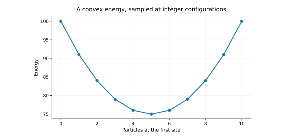
This proof does not require positive definiteness. Nor does it imply that an ascent algorithm reaches a global maximum. Section 7 will display strict local traps despite the validity of Theorem 2.5.
Lemma 2.6 (Occupied neighbors cannot both be ascent-stationary). If \(K(p,p)=K(q,q)=\kappa\) and \(K(p,q)<\kappa\), an ascent-stationary configuration cannot occupy both endpoints of the edge \(pq.\)
Proof. If \(c(p),c(q)>\) 0, both directed moves are admissible and
At least one increment is positive, contradicting stationarity.\(\square\)
Thus an ascent-stationary support is an independent set of the move graph under the attractive diagonal-gap condition. In particular, on a complete graph every terminal configuration is a Dirac configuration, with no small-parameter assumption. On a sparse graph, an independent set may have several vertices; the missing step is to exclude those separated clusters.
3 The geometric class: an atlas of admissible graphs
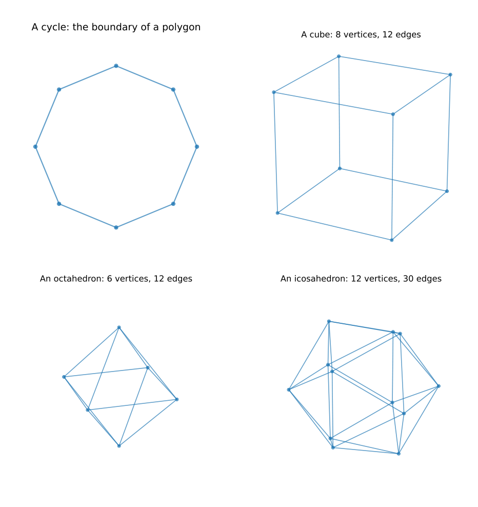
3.1 Inscribed convex hulls and their edge graphs
Choose distinct vectors \(v_{x}\in \mathbb{R}^{m}\), indexed by \(x\in X\), such that
Their convex hull \(P=\operatorname{conv} \{v_{x}:x\in X\}\) is considered in its affine span. Every \(v_{x}\) is a vertex: the functional \(z\mapsto \langle v_{x},z\rangle\) has value \(R^{2}\) at \(v_{x}\) and strictly smaller values at all other listed points. Let \(\mathcal{E}_{P}\) be the set of its one-dimensional faces, called edges.
Definition 3.1 (A compatible spherical move graph). The embedded graph \((G,(v_{x})_{x\in X})\) is compatible if
The graph may have additional edges, but it has exactly the same vertex set as the convex hull.
This is a condition on a graph together with an embedding, not merely on a drawing. A different drawing of the same abstract graph may change which pairs are convex-hull edges and may change the kernel. Inscribability itself is a substantial subject in convex geometry; not every polytope has an inscribed realization [8, 9]. Our theorems assume a realization rather than attempting to characterize all inscribable graphs.
The interaction will be
It is often better to remove the irrelevant constant factor \(e^{\beta R^{2}}\). Define
By Theorem 2.4, both kernels induce exactly the same accepted moves. The quantity \(a_{xy}\) is a squared Euclidean chord length; it is not, in general, a metric and is not the graph distance.
3.2 Families beyond regular polyhedra
A cycle \(C_{M},M\ge 3\), can be realized by any \(M\) distinct points on a circle in their cyclic order. Unequal angular gaps are allowed. Cartesian products of inscribed polytopes are again inscribed: if \(\|u\|=R_{1}\) and \(\|w\|=R_{2}\), then \(\|(u,w)\|^{2}=R_{1}^{2}+R_{2}^{2}\). Their edges change only one factor at a time. This yields products of cycles with unequal lengths, rectangular boxes, and hypercubes. A proof of the edge statement is included in Section 5.
Corollary 3.2 (Hamiltonian graphs admit a compatible kernel). If a finite graph with \(M\ge 3\) has a Hamiltonian cycle, it has a compatible spherical realization in \(\mathbb{R}^{2}.\)
Proof. Label the vertices \(x_{0},...,x_{M-1}\) in the order of a Hamiltonian cycle, and set \(v_{x_{j}}=(\operatorname{cos} (2\pi j/M),\operatorname{sin} (2\pi j/M))\). The convex-hull edges are precisely the consecutive pairs on this cycle, all of which are graph edges. Other graph edges are allowed chords.\(\square\)
The kernel in this corollary is adapted to the chosen cycle. It is not intrinsically determined by the abstract graph, and it should not be replaced silently by \(e^{-\beta d_{G}}.\)
The nonperiodic grid example is worth spelling out. In an \(r\times s\) grid with \(r,s\ge 2\) and \(r\) even, reserve the first column for the return path. Traverse the first row, then snake down successive rows through columns 2\(,...,s\), finally return up the reserved first column. This visits every
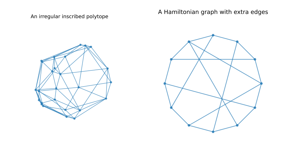
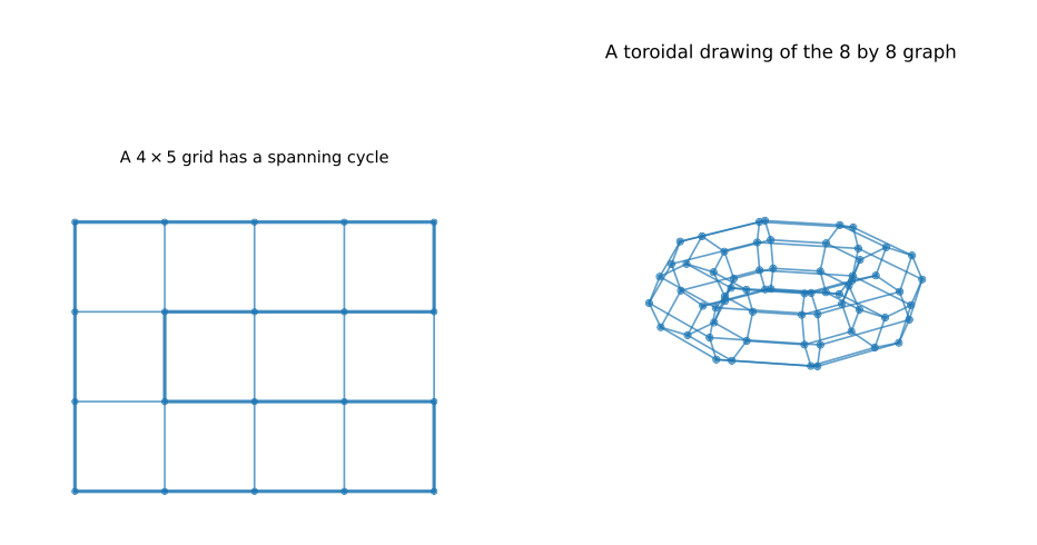
vertex once and closes the cycle. If instead \(s\) is even, interchange the coordinates. Consequently these rectangular grids are covered by Theorem 3.2, with a circularly designed kernel. Their ordinary planar coordinates, which include non-extreme interior vertices, do not themselves satisfy Theorem 3.1.
3.3 The linear-functional lemma
The proof of concentration rests on one elementary polyhedral fact. We give the geometric argument explicitly so that the role of the skeleton condition is visible.
Lemma 3.3 (Edge directions generate the vertex cone). Let \(P\) be a convex polytope and \(p\) one of its vertices. For every \(x\in P\), the vector \(x-p\) is a nonnegative linear combination of the vectors \(q-p\), where \(pq\) runs over the edges incident to \(p.\)
Proof. Work in the affine span translated to \(p=0\). There is a linear functional \(h\) strictly positive at every other vertex of \(P\); one can take a functional strictly exposing \(p\) and change its sign. Choose 0 \(<\epsilon <\min_{v\ne p}h(v)\) and cut \(P\) by \(h=\epsilon\). Its section \(Q\) is a polytope. Every vertex of \(Q\) lies on an edge of \(P\) that crosses this hyperplane. To justify this assertion, let \(F\) be the smallest face of \(P\) containing such a point in its relative interior. The hyperplane cuts the relative interior of \(F\), so the local dimension of \(F\cap \{h=\epsilon \}\) is dim \(F-1\). A vertex of the section has dimension zero, hence dim \(F=1\). The only original vertex below the hyperplane is \(p\), so every crossing edge is incident to \(p.\)
Thus the vertices of \(Q\) are points \(t_{q}q\) with \(t_{q}>0\) and \(pq\) an incident edge. For a nonzero \(x\in P,\) write \(x=\sum _{v\ne p}\lambda _{v}v\) with \(\lambda _{v}\ge\)0 (a coefficient at \(p=\) 0 may be omitted). Then
The coefficients on the right sum to one, and each point \(\epsilon v/h(v)\) lies on the segment \([p,v]\) and in the section \(Q\). Thus the ray through \(x\) meets \(Q\). This intersection is a convex combination of its vertices \(t_{q}q\). Rescaling gives the desired nonnegative combination of edge directions. The case \(x=p\) is immediate.\(\square\)
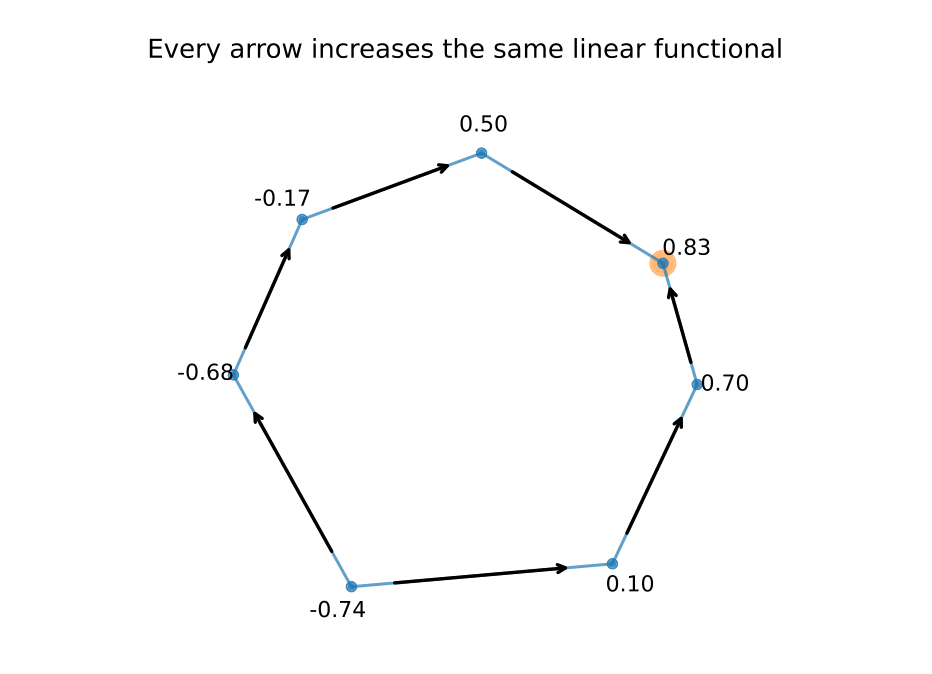
Lemma 3.4 (Strict local maxima of linear functions). Let \(\ell\) be linear on the affine span of a polytope. If a vertex \(p\) satisfies \(\ell (p)>\ell (q)\) at every adjacent vertex \(q\), then \(\ell (p)>\ell (x)\) for every other vertex \(x\). In particular, there is at most one strict local maximum on the edge graph.
Proof. For \(x\ne p,\) Theorem 3.3 gives \(x-p=\sum _{q\sim _{P}p}\alpha _{q}(q-p)\) with \(\alpha _{q}\ge 0\) and at least one nonzero coefficient. Therefore
Non-strict local maxima require care: an exposed edge or face can consist of several maximizers. The small-parameter stationarity estimate below will provide a strict quantitative gap, precisely eliminating that ambiguity.
4 Universal concentration on compatible spherical graphs
4.1 An explicit theorem
Fix a compatible spherical realization and \(n\ge\)2. Set
Both \(A\) and \(\delta\) are computed from the embedding. In particular, 0 \(<\delta \le A\le 2R^{2}\). The constants do not depend on an initial occupation field.
Theorem 4.1 (Small-parameter concentration). Assume (3.1) and (3.2). For
the only ascent-stationary configurations for \(K_{\beta}\) or \(\overline{K}_{\beta}\) are \(n\delta _{x},x\in X\). Every complete ascent trajectory therefore terminates at a single cluster, from every initial \(c^{0}\in \mathcal{C}_{n}.\)
More quantitatively, every non-Dirac configuration admits a move along a convex-hull edge for which
What is and is not uniform
For fixed \(G\), its embedding, and \(n\), the theorem covers every initial arrangement and every complete sequence of improving moves. It does not select the terminal vertex. The sufficient threshold shrinks when \(n\) grows or when the geometry develops very short edges. It is not asserted to be the largest possible threshold. At \(\beta =0\) the kernel is constant and every increment is zero, so the strict inequality \(\beta >\) 0 is essential.
4.2 Uniform control of the exponential remainder
Lemma 4.2 (A quantitative first-order increment). Define
For every admissible pair \((p,q)\) and every \(\beta >0,\)
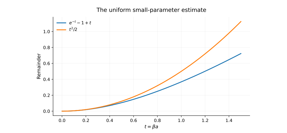
Proof. For \(t\ge\)0, the integral remainder formula gives
Hence, for \(a,a^{\prime}\in [0,A]\), both remainders lie in \([0,\beta ^{2}A^{2}/2]\), and
Using a bound of \(\beta ^{2}A^{2}\) here would also work, but would lose a factor of two. With \(r=c-\delta _{p},\) (2.5) and the constant unit diagonal give
The linear contribution is
The remaining term has absolute value at most 2\((\sum _{y}r(y))\beta ^{2}A^{2}/2=(n-1)\beta ^{2}A^{2}\). This bound is uniform over configurations, edges and schedules.\(\square\)
4.3 Proof of concentration
Proof of Theorem 4.1. Suppose first that \(c\) is ascent-stationary. At every occupied \(p\) and every convex-hull neighbor \(q,\) Theorem 4.2 implies
Dividing by 2\(\beta >\) 0 and using (4.2) gives
But \(S_{c}\) is the restriction of the single linear functional \(v\mapsto \langle v,b_{c}\rangle\) to the vertices of \(P\). By Theorem 3.4, it has at most one strict local maximum on the skeleton. Since every occupied vertex is such a maximum, the support of \(c\) has one element.
Conversely, every \(n\delta _{x}\) globally maximizes the energy by Theorem 2.5, because \(a_{xy}>0\) for \(x\ne y\). Hence it is ascent-stationary. Finite termination now follows from Theorem 2.3.
For the quantitative assertion, take a non-Dirac \(c\). The linear functional \(S_{c}\) cannot have a strict local maximum at every occupied vertex, because there are at least two occupied vertices. Choose one, \(p\), which is not a strict local maximum. There is a convex-hull neighbor \(q\) with \(S_{c}(q)\ge S_{c}(p).\) Then
This proves (4.3).\(\square\)
The proof uses no hypothesis that \(b_{c}\ne 0\). If \(b_{c}=0\), then \(S_{c}\) is constant, and (4.5) itself supplies a strictly positive increment from any occupied vertex along any convex-hull edge in the stated regime. Thus a symmetric or “balanced” initial configuration is not an excluded exceptional case.
Corollary 4.3 (A move bound for global steepest ascent). Under the hypotheses of Theorem 4.1, global steepest ascent terminates after at most
accepted moves.
Proof. Before the terminal Dirac state, the largest admissible increment is at least \(\beta \delta\). The energy at termination is \(n^{2}\). In labeled coordinates, the \(n\) self-interactions equal one, and each of the \(n(n-1)\) other interactions is at least \(e^{-\beta A}\). Hence
Finally, 1 \(-e^{-t}\le t\) for \(t\ge 0.\quad \square\)
This bound concerns global steepest selection. A source-by-source algorithm may choose an improving move whose gain is smaller than \(\beta \delta\), so (4.8) must not be applied to it without an additional argument. Such an algorithm still terminates at a single cluster by the stationary-state theorem.
4.4 Perturbing the interaction, not just the geometry
Let \(B:X\times X\to \mathbb{R}\) be symmetric, with no separability or smoothness assumption. Consider
Its diagonal need not be constant, so the full increment (2.4) must be used.
Theorem 4.4 (Uniform robustness). Under the geometric hypotheses of Theorem 4.1, suppose
Then every non-Dirac configuration has an admissible move with strictly positive \(\widetilde{K}_{\beta}\)-energy increment. Consequently every complete ascent implementation terminates at a Dirac configuration.
Proof. Set \(\epsilon =\|B\|_{\infty}\) and \(H=\widetilde{K}_{\beta}-\overline{K}_{\beta}\). The mean value theorem yields
Applying (2.5) to \(H\), with \(\sum r=n-\)1, gives
The extra 2\(\|H\|_{\infty}\) controls the possibly nonconstant diagonal. The hypotheses imply
so \(e^{\beta \epsilon}\le e\). Given a non-Dirac \(c\), select the move from (4.3). Then
No non-Dirac state can therefore be stationary. Finiteness and completeness finish the proof.\(\square\)
Remark 4.5 (Scope of the robust conclusion). A varying diagonal can give different energies to different Dirac configurations. The theorem guarantees concentration, not selection of the best vertex for that perturbed energy. It also does not assert that \(\widetilde{K}_{\beta}\) is positive definite. The spectral descent results below impose their own coercivity hypotheses; ascent robustness does not supply them automatically, especially uniformly as \(\beta \downarrow 0.\)
4.5 The structural template behind the proof
The spherical theorem is a convenient way to verify a more abstract criterion. Suppose \(\sigma (x,y)=\sigma (y,x)\) has constant diagonal \(\sigma _{\ast}\), satisfies \(\sigma (x,y)\le \sigma _{\ast}\), and has a positive edge gap on a spanning connected subgraph \(H\subseteq G\). Let \(S_{c}(x)=\sum _{y}c(y)\sigma (x,y)\). Assume that for every \(c\in \mathcal{C}_{n}\), the function \(S_{c}\) has at most one strict local maximum on \(H\). With \(a_{xy}=\sigma _{\ast}-\sigma (x,y)\), the expansion and strict-gap proof above apply verbatim. The convex-hull condition is valuable because it verifies the local-maximum property simultaneously for all occupation fields, without checking an exponentially large state space.
5 Recovering the discrete torus and its Fourier structure
5.1 The torus is a product of polygons
Let
with nearest-neighbor moves \(x\mapsto x\pm e_{j}\) modulo \(N\). Define
Then \(\|v_{x}\|^{2}=d\) and
Thus the original interaction is exactly \(e^{\beta \langle v_{x},v_{y}\rangle}.\)
To identify the skeleton, let \(Q_{N}\) be the regular \(N\)-gon. The convex hull in (5.1) is \(Q_{N}^{d}\). The equality follows because a product of convex combinations can be expanded as a convex combination of product vertices; the reverse inclusion is immediate. A face exposed by a functional \((\ell _{1},...,\ell _{d})\) is the product of the faces exposed in the separate factors. Dimensions add. Hence a onedimensional face is one polygon edge times vertices in all other factors. The skeleton is exactly
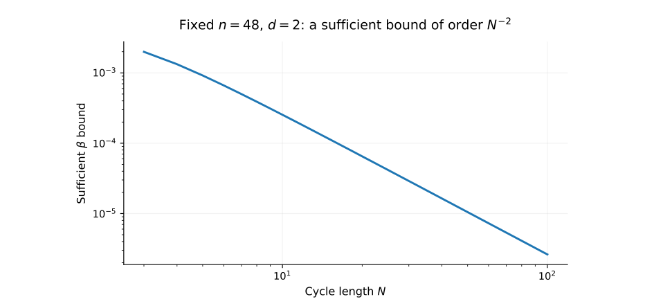
Corollary 5.1 (An explicit torus concentration bound). For the original unperturbed torus kernel, every complete ascent trajectory concentrates if
Global steepest ascent then satisfies
Proof. On every nearest-neighbor edge, \(a_{pq}=\delta _{N}:=1-\operatorname{cos} (2\pi /N)\), while \(A\le 2d\). Use Theorems 4.1 and 4.3. A sharper bound can be obtained by retaining the exact \(A\) instead of 2\(d.\quad \square\)
For \(N=2\), the simple move graph is the \(d\)-dimensional hypercube; use the embedding \(x\mapsto ((-1)^{x_{1}},...,(-1)^{x_{d}})\). The same reasoning applies with \(\delta =2\) and \(A=2d\). For \(N=1\) there is one vertex and concentration is tautological. Products with different cycle lengths are handled by replacing \(\delta _{N}\) by the smallest factor gap and \(A\) by the total maximum dissimilarity. For hypercubes one also has the all-parameter complete graph observation only in dimension one; higher-dimensional cubes are not complete graphs.
5.2 The original separable perturbation is included
Let \(f_{j}\in C^{2}(\mathbb{R}/\mathbb{Z})\) be even and write
We use 1-periodic functions here; a 2\(\pi\)-periodic convention is identical after rescaling the arguments. Evenness makes the kernel symmetric. Define \(B(x,y)=\sigma _{\eta}(x,y)-\sigma _{0}(x,y)\). Then
Theorem 4.4 therefore yields the explicit sufficient conditions
This recovers perturbative concentration from all initial configurations without requiring a separate nonvanishing-mode assumption. For this particular conclusion, \(C^{2}\) regularity is more than is needed: a uniform bound on the sampled perturbation suffices. The smoothness assumption remains relevant to the continuous-profile results in Section A.
5.3 First modes are coordinates of the geometric barycenter
Define the unnormalized first Fourier modes by
The \(j\) th pair of coordinates of \(b_{c}\) is \((\Re A_{j}(c),-\Im A_{j}(c))\). Consequently
For the unnormalized kernel, Taylor expansion gives
where the remainder is uniform for fixed \(n,N,d\). Indeed, \(\sum _{x,y}c(x)c(y)\langle v_{x},v_{y}\rangle =\|b_{c}\|^{2}\), and \(|\langle v_{x},v_{y}\rangle |\le d\) controls the exponential remainder. For the normalized kernel, the first-order term is instead \(\|b_{c}\|^{2}-dn^{2}\); the difference is constant on \(\mathcal{C}_{n}.\)
The “bad” set
marks a loss of the one-dimensional cosine profile in that coordinate. It is not an obstruction to the geometric proof. If \(A_{j}(c)=0\), then \(S_{c}\) is constant along \(j\) th-coordinate edges, which is incompatible with (4.7) at an occupied site. Only the terminal configuration needs to be excluded from \(B_{N}\); there is no need to assert that the trajectory never crosses this set.
5.4 Positive definiteness and the exact Fourier convention
Proposition 5.2 (Strict positivity of the exponential Gram kernel). For distinct vectors \(v_{x}\in \mathbb{R}^{m}\) and \(\beta >0\), the matrix \(K_{\beta}(x,y)=e^{\beta \langle v_x,v_y\rangle}\) is strictly positive definite. For an equal-radius embedding, the same holds for \(\overline{K}_{\beta}.\)
Proof. For real coefficients \(u_{x}\), expand the exponential absolutely:
At \(k=0\), the tensor is the scalar \(\sum _{x}u_{x}\). If the left side is zero, every nonnegative summand is zero. Therefore \(\sum _{x}u_{x}p(v_{x})=0\) for every polynomial \(p\), because tensor coordinates contain all monomials. For a fixed \(z\in X\), use the polynomial
It equals one at \(v_{z}\) and zero at every other \(v_{y}.\) Hence \(u_{z}=0.\) Since \(z\) was arbitrary, the quadratic form is strictly positive away from the origin. Multiplication by \(e^{-\beta R^{2}}>0\) preserves this property.\(\square\)
For the torus, set \(k(z)=K_{\beta}(z,0)\) and use the unnormalized transform
Orthogonality of the characters gives
For completeness, applying \(K\) to the character \(\chi _{m}(x)=e^{2\pi i\langle m,x\rangle /N}\) gives
Thus \(\widehat k(m)\) are exactly the eigenvalues. By Theorem 5.2 they are strictly positive. The factor \(M^{-1}\)
in Parseval is crucial; it is absent from the eigenvalues themselves.
Small perturbations of the matrix preserve this positivity for each fixed \(\beta >0\) by continuity of eigenvalues. This does not imply one perturbation size works uniformly for all \(\beta \downarrow 0\), since \(K_{0}\) has rank one. The concentration bound (5.6) does not rely on such a uniform spectral claim.
6 Trees: a different kernel and an exact threshold
6.1 Intrinsic distance rather than an embedding
Let \(G\) be a finite tree with unit-length edges. We now choose
No spherical realization is assumed. The diameter is \(D=\) diam \(G\). This is a second model, not a reinterpretation of the spherical theorem.
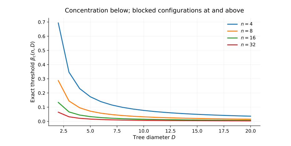
Theorem 6.1 (Sharp universal concentration threshold on trees). Let \(n\ge 4\) and \(D\ge 2\), and put
The following are equivalent:
(i) Every complete ascent trajectory from every configuration in \(\mathcal{C}_{n}\) terminates at a Dirac configuration.
(ii) Every ascent-stationary configuration is a Dirac configuration.
(iii) 0 \(<\beta <\beta _{c}(n,D).\)
If \(n\le 3\), concentration holds for every \(\beta >0\) on every finite tree. It also holds for every \(\beta >0\) and every \(n\) when the tree has at most two vertices.
6.2 An occupied leaf provides the improving move
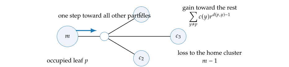
Proof of sufficiency in Theorem 6.1. Suppose \(c\) has at least two occupied sites. Let \(H\) be the smallest subtree containing its support: equivalently, the union of the unique paths joining occupied vertices. Every leaf of \(H\) is occupied, since an unoccupied leaf could be removed without losing the support. The subtree has at least two leaves. At least one occupied leaf, \(p\), has occupation
Indeed, two leaves each carrying more than \(n/\)2 particles would already exceed the total mass.
Let \(q\) be the unique neighbor of \(p\) in \(H\). Every path from \(p\) to any other occupied \(y\) starts with \(pq\), so
The leave-one-out formula gives the exact expression
Since 1 \(\le d_{G}(p,y)\le D\) and 0 \(<r<1,\)
The function \((m-1)/(n-m)\) is increasing for 1 \(\le m<n\), as follows by differentiating its real extension or cross-multiplying consecutive values. Since \(m\le a\) and \(n-a=b\), the right side is positive if
which is precisely \(\beta <\beta _{c}(n,D)\). Every non-Dirac configuration therefore has an improving move and cannot be stationary.
When \(n=2\) or 3, the selected leaf has \(m=1\), so the negative term in (6.3) vanishes and the increment is positive for every \(\beta >0\). For \(n=1\) every configuration is already a Dirac. A one-vertex graph is trivial, and a two-vertex tree is complete, so Theorem 2.6 applies for every \(n.\) Termination was proved in Theorem 2.3.\(\square\)
6.3 Two endpoint clusters prove sharpness
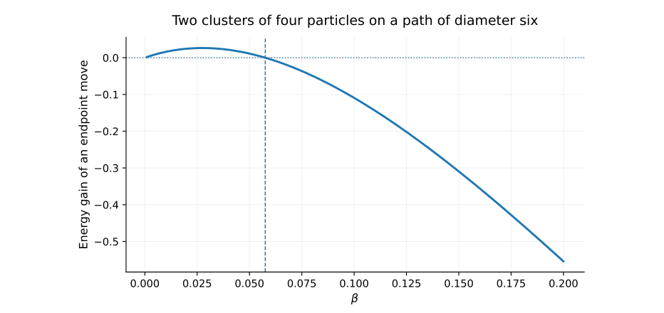
Proof of necessity and equivalence in Theorem 6.1. Let \(x,y\) be endpoints of a diameter, so \(d_{G}(x,y)=D\). Both are leaves of the whole tree: any additional edge leaving an endpoint off the diametral path would create a longer path. Consider
There are exactly two admissible directed moves from occupied sites, each toward the other cluster. Their increments are
If \(\beta \ge \beta _{c}\), then \(r^{D-1}\le (a-1)/b\), making the first increment nonpositive. The second is nonpositive as well, because
which is equivalent to \(a(a-1)\le b(b-1)\) and follows from \(a\le b\). Thus a non-Dirac stationary state exists. At equality in the threshold, a zero increment is still rejected, so the boundary value belongs to the non-universal regime.
Statement (ii) implies (i) by finite termination. Conversely, if a non-Dirac stationary state exists, using it as the initial state violates (i). The sufficient and necessary parameter conditions established above complete all equivalences.\(\square\)
Corollary 6.2 (A quantitative steepest bound on a tree). Under the subcritical hypotheses of Theorem 6.1, set
Global steepest ascent takes at most \((n^{2}-E_{K}(c^{0}))/g\) accepted moves. For \(n=2,3\), use \(a=1,b=n-1,\) giving \(g=2(1-r)(n-1)r^{D-1}.\)
Proof. The lower bound (6.4) is decreasing as a function of \(m\), so it is at least its value at \(m=a.\) Every non-Dirac state has a move of gain at least \(g\). Sum this gain along global steepest ascent and use the maximum energy \(n^{2}.\quad \square\)
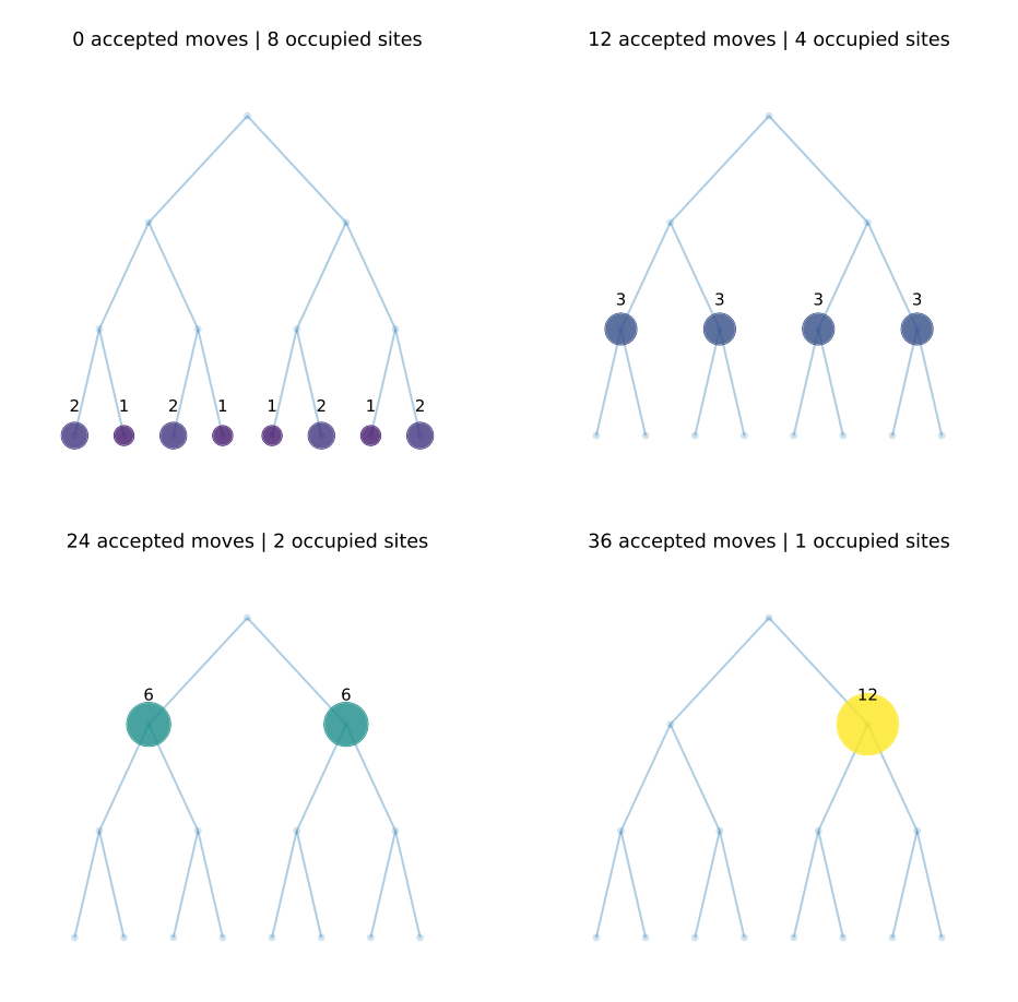
Animation 2. tree_ascent.mp4. The offline companion gallery.html provides playback and a state-by-state slider.
7 Why the graph and the kernel must be considered together
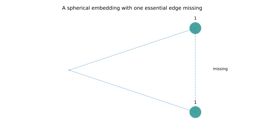
7.1 Removing one geometrically essential edge
Consider the path \(p-q-r\) and the three unit vectors
With \(K_{\beta}(x,y)=e^{\beta \langle v_{x},v_{y}\rangle}\), put one particle at \(p\) and one at \(r\). The only allowed destinations are \(q.\) Since
each move has increment
The configuration is therefore strictly blocked for every positive parameter. All three points lie on a circle, the graph is connected, and the exponential Gram matrix is strictly positive definite. What fails is precisely (3.2): the convex hull is a triangle, but the edge \(pr\) is missing from the move graph.
This example does not contradict the tree theorem: that theorem uses \(e^{-\beta d_{G}}\), not the dot products in (7.1).
7.2 The same cycle, a different kernel
On the cycle \(C_{6}\), number the vertices 0\(,1,...,\) 5 and choose
Use now \(K_{\beta}(x,y)=r^{d_{C_6}(x,y)},r=e^{-\beta}\). Every admissible increment has the same value by the rotations and reflections that preserve the configuration. For the move 0 \(\to 1,\)
since 2\(r(1-r)\le 1/2\). This proves non-Dirac stationarity for every \(\beta >0\), including arbitrarily small ones.
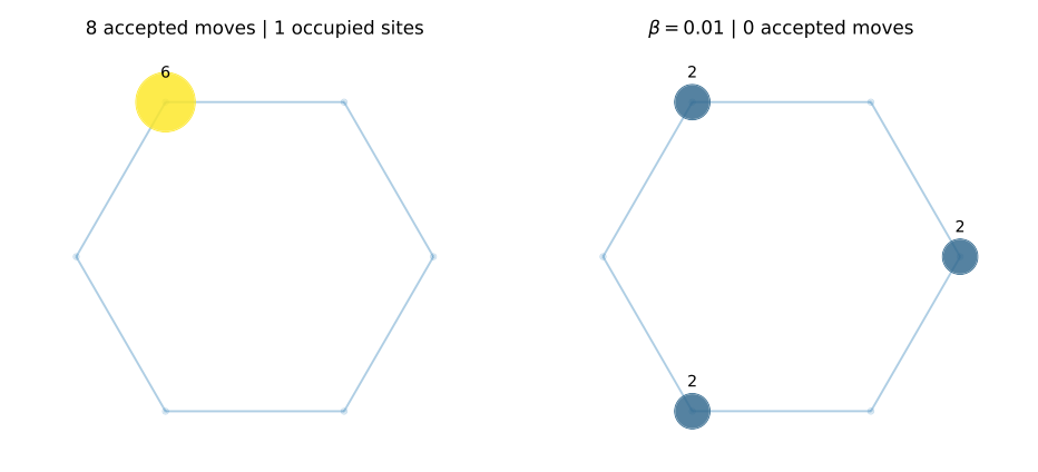
By contrast, with the regular-circle embedding \(v_{j}=(\operatorname{cos} (2\pi j/6),\operatorname{sin} (2\pi j/6))\) and the normalized spherical kernel, \(A=2,\delta =1/2\) and \(n=6\). The sufficient bound is \(\beta \le 1/40\). Hence the identical initial occupation (7.3) must concentrate when, for example, \(\beta =0.01.\)
Animation 3. cycle_ascent.mp4. The offline companion gallery.html provides playback and a state-by-state slider.
A hierarchy of conclusions
Finiteness plus strict energy improvement gives termination. A strict diagonal maximum makes Dirac configurations global maximizers. Neither statement excludes non-Dirac local traps. Universal concentration requires a further compatibility mechanism: the polyhedral linearization, the tree leaf argument, completeness of the move graph, or another independently verified condition.
7.3 Strictly improving asynchronous moves are part of the model
On a two-vertex graph, put one particle at each vertex and take \(K(p,p)=K(q,q)=1,K(p,q)=r<1\). Each particle, considered alone, can join the other with gain 2\((1-r)>0\). If both particles simultaneously act on the old configuration, they merely exchange positions. The occupation field and energy do not change. Repeating this synchronous operation makes labeled particles oscillate and does not reproduce the ascent algorithm.
The same issue explains why zero-gain moves are rejected. Allowing them can create cycles on a finite energy plateau. A modified rule might intentionally traverse such plateaus, but its termination proof and threshold statements would have to be reformulated.
8 Repulsive dynamics: what survives on a general graph
8.1 Three distinct notions of dispersion
Descent is not simply ascent with a different terminal answer. It is useful to separate three questions. How unequal can occupations of neighboring sites be? How far is the whole occupation vector from a relaxed minimizer? How many pairs of particles can be too close? The following results address these questions through different hypotheses, and they should not be conflated.
The graph in this section is an arbitrary finite connected simple undirected graph unless a special case is explicitly stated.
8.2 Neighboring-occupation rigidity
Assume first that the diagonal is constant, \(K(x,x)=\kappa\). For an edge \(pq\), define
with \(B_{pq}=\) 0 if the maximum is over an empty set.
Theorem 8.1 (A graph-local rigidity criterion). Let \(n\ge 2\). If every edge satisfies
then every descent-stationary configuration satisfies
Consequently
Proof. Suppose \(c(p)-c(q)\ge 2\). In particular, the move \(p\to q\) is admissible. Separate the \(y=p,q\) terms in the potential difference:
The two endpoint occupations sum to at least two, so the remaining mass is at most \(n-2.\) Therefore
Equation (2.6) now gives \(\mathcal{D}_{p,q}E_{K}(c)=2[-(V_{c}(p)-V_{c}(q))+\alpha _{pq}]<0\), contradicting descent stationarity. Exchange \(p\) and \(q\) for the opposite inequality. Summing (8.3) along a shortest path gives (8.4).\(\square\)
Corollary 8.2 (A simple diagonal-dominance bound). If 0 \(\le K(x,y)\le b<\kappa\) for \(x\ne y\), then
implies the conclusion of Theorem 8.1.
Proof. Here \(\alpha _{pq}\ge \kappa -b\) and \(B_{pq}\le b\). Thus \(\kappa >(n-1)b\) implies \(\alpha _{pq}>(n-2)B_{pq}\). The sharper bound \(B_{pq}\le b\), rather than 2\(b\), uses nonnegativity of the off-diagonal entries.\(\square\)
For the unperturbed torus kernel, \(\kappa =e^{\beta d}\) and \(b=e^{\beta (d-\delta _{N})}\). Hence, for \(n\ge 2,\)
is sufficient. When \(n=2\), the numerator is zero and every \(\beta >0\) works. The stronger original condition \(\kappa -b>nb\), equivalent to \(\beta >\operatorname{log} (n+1)/\delta _{N}\), is also sufficient; (8.6) simply retains the sharper remaining-mass estimate \(n-2.\)
For the graph-distance kernel on any connected unit-edge graph, let \(r=e^{-\beta}\). Adjacent \(p,q\) satisfy \(|d_{G}(p,y)-d_{G}(q,y)|\le\)1. If \(y\notin \{p,q\}\), both distances are at least one. Thus
The sufficient condition becomes
For \(n\ge 4\) this is \(\beta >\operatorname{log} (n-2)\); for \(n=2,3\) it holds for every \(\beta >0\). For \(n=1\), neighboring occupations differ by at most one without any hypothesis.
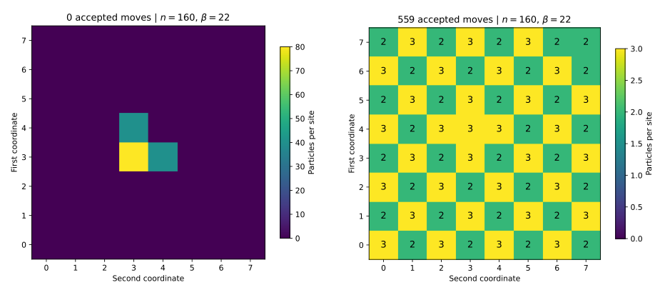
Animation 4. torus_descent.mp4. The offline companion gallery.html provides playback and a state-by-state slider.
8.3 The relaxed minimizer and spectral discrepancy
The continuous relaxation keeps the same energy but allows \(c\in \mathbb{R}_{\ge0}^{X}\) with total mass \(n\). It is used only as a comparison problem; the algorithm still moves integer particles. Define
This is the smallest eigenvalue of the compression of \(K\) to \(\mathcal{H}\). The subspace need not be invariant under \(K\) unless an additional condition such as constant row sums is imposed.
Theorem 8.3 (Uniform reference state under constant row sums). Suppose \(K\mathbf1=s\mathbf1\) and \(\lambda _{H}>0.\) Then \(\overline{c}=(n/M)\mathbf1\) is the unique relaxed minimizer and, for every \(c\) of total mass \(n,\)
Along every descent trajectory,
Proof. Write \(c=\overline{c}+g\), where \(g\in \mathcal{H}\). Expanding the energy gives
Symmetry and the row-sum condition imply \(\overline{c}^{\top}Kg=(n/M)(K\mathbf1)^{\top}g=(ns/M)\sum _{x}g(x)=0\). The definition of \(\lambda _{H}\) proves (8.8). Strict positivity forces equality only when \(g=0\), proving uniqueness. Taking square roots, using \(\|g\|_{\infty}\le \|g\|_{2}\), and using energy monotonicity proves (8.9).\(\square\)
In particular, for any two sites,
The uniform relaxed vector need not be an integer configuration when \(M\) does not divide \(n\). This is not an inconsistency: it remains a valid energy lower bound and reference vector.
For a translation-invariant torus kernel,
These identities follow from (5.12)–(5.13) and recover the original Fourier estimate, with the same normalization.
Theorem 8.4 (The nonuniform reference state). Suppose only that \(K\) is symmetric and \(\lambda _{H}>0\). The relaxed problem has a unique minimizer \(c_{\ast}\), and
for every feasible \(c\). Thus (8.9) remains true with \(\overline{c}\) replaced by \(c_{\ast}\). If \(K\) is invertible and \(K^{-1}1\) is componentwise positive with 1 \(\top K^{-1}1>0\), then
Proof. The feasible simplex is compact, so a minimizer exists. On the mass hyperplane, every nonzero feasible direction belongs to \(\mathcal{H}\), on which the Hessian 2\(K\) is positive definite. The energy is therefore strictly convex on this hyperplane, so the minimizer is unique. For a feasible \(c\), the segment \(c_{\ast}+t(c-c_{\ast})\) is feasible for 0 \(\le t\le\)1. Its right derivative at \(t=\) 0 is nonnegative:
Expanding around \(c_{\ast}\) and using \(c-c_{\ast}\in \mathcal{H}\) gives
This argument remains valid if \(c_{\ast}\) has zero coordinates. Under the last hypotheses, the vector in (8.12) is feasible and satisfies \(Kc_{\ast}=\lambda 1\) for a scalar \(\lambda\). The first-order term then vanishes for every mass-preserving direction, so strict convexity identifies it as the minimizer.\(\square\)
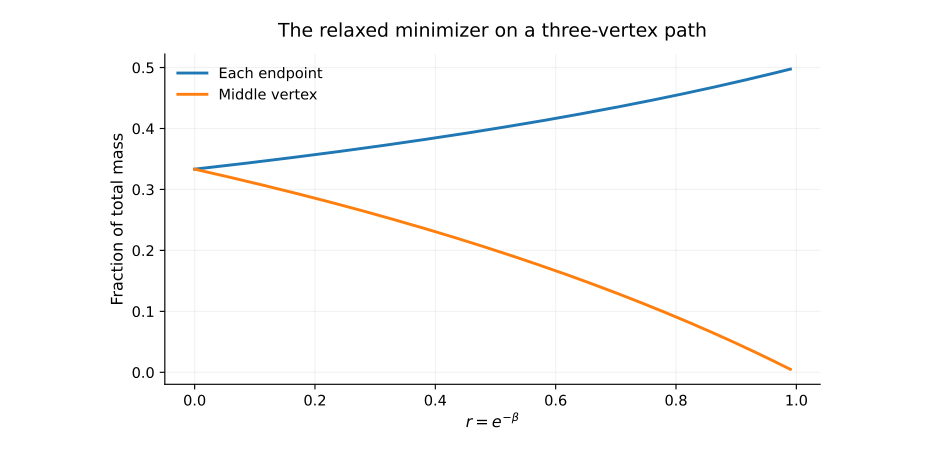
Example 8.5 (An irregular graph need not prefer uniformity). On the three-vertex path with
Its leading principal minors are 1, 1\(-r^{2}\) and \((1-r^{2})^{2}\), so it is positive definite. Direct multiplication gives
Hence
which is nonuniform for \(r>0\). The row sums 1 \(+r+r^{2},1+2r,1+r+r^{2}\) are not equal. It would therefore be wrong to replace Fourier by eigenvalues while keeping the uniform minimizer without checking the row-sum hypothesis.
8.4 Large-parameter asymptotics
The original large-\(\beta\) spectral estimate has a matrix form that does not use Fourier analysis.
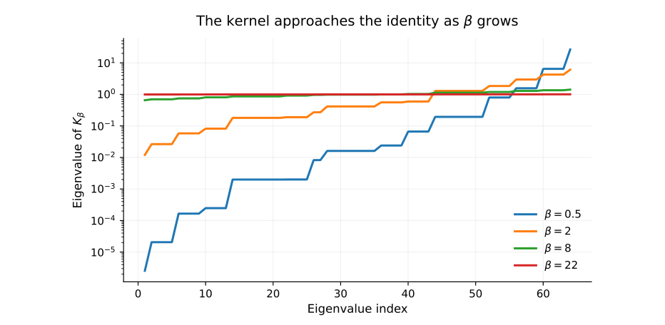
Proposition 8.6 (Near-diagonal kernels). Assume \(\overline{K}_{\beta}(x,y)=e^{-\beta a_{xy}}\), with \(a_{xx}=0,a_{xy}=a_{yx}\) and \(\gamma :=\min_{x\ne y}a_{xy}>0\). Suppose the row sums are constant for each \(\beta\). For fixed \(M,n,c^{0},\)
The unnormalized kernel \(e^{\beta \sigma (x,y)}\), with constant diagonal exponent \(\sigma _{\ast}\) and \(a_{xy}=\sigma _{\ast}-\sigma (x,y)\), has \(\lambda _{H}=e^{\beta \sigma _{\ast}}(1+O(e^{-\beta \gamma}))\) and the same ratio (8.15).
Proof. Write \(\overline{K}_{\beta}=I+R_{\beta}\). The diagonal of \(R_{\beta}\) is zero and every off-diagonal entry is at most \(e^{-\beta \gamma}\)
in absolute value. For every \(g,\)
where the last inequality follows from \((\sum _{x}|g(x)|)^{2}\le M\|g\|_{2}^{2}\). Taking infima over nonzero \(g\in \mathcal{H}\) proves
For a nonnegative \(c\) of mass \(n,\)
Apply this identity to \(c^{0}\) and \(\overline{c}\), subtract, and divide by 1 \(+O(e^{-\beta \gamma})\). The division is valid for all sufficiently large \(\beta\), since the lower bound for \(\lambda _{H}\) is then positive. Scaling by \(e^{\beta \sigma _{\ast}}\) proves the final assertion.\(\square\)
For the torus, \(\gamma =\delta _{N}\) and \(\sigma _{\ast}=d\), recovering
The constants hidden in \(O(\cdot )\) may depend on \(M,n,c^{0}\) and the fixed geometry; no uniformity under mesh refinement is claimed.
8.5 Pair-separation estimates along the whole trajectory
Let \(\sigma :X\times X\to \mathbb{R}\) be symmetric with constant diagonal \(\sigma (x,x)=\sigma _{\ast}\). For \(K_{\beta}=e^{\beta \sigma}\), follow a labeled realization \(x_{1}(t),...,x_{n}(t)\) of a descent trajectory. Assume \(n\ge\)2 and define
Labels are used only to count unordered pairs. The conclusion depends only on the occupation field.
Theorem 8.7 (A quantitative close-pair bound). For every real \(s\) and every accepted-move index \(t,\)
In particular, if \(s>s_{0}\) and
then \(P_{s}(t)=0\) at every step. Pairwise distinct initial particles are needed only when one wishes to infer collision exclusion using \(s=\sigma _{\ast}\) and a strict off-diagonal maximum.
Proof. The diagonal contribution is constant, so
Descent implies \(E_{K}(c^{t})\le E_{K}(c^{0})\), and at time zero every off-diagonal particle interaction is at most \(e^{\beta s_{0}}\). Therefore
Dividing gives (8.16). Under (8.17), its right-hand side is strictly less than one, and the nonnegative integer \(P_{s}(t)\) must vanish.\(\square\)
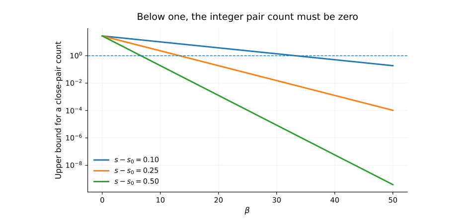
For \(\sigma =-d_{G}\), if the initial particles are pairwise distinct and \(r_{0}=\operatorname{min} i_{<j}d_{G}(x_{i}(0),x_{j}(0))\), the bound reads
Because unit-edge graph distances are integers, taking \(r=r_{0}-1\) shows that \(\beta >\operatorname{log} \binom n2\) prevents the minimum distance from ever falling below its initial value. This is a lower bound, not a claim that the minimum distance is monotone at every move.
For a spherical embedding, \(\sigma (x,y)=R^{2}-\|v_{x}-v_{y}\|^{2}/2\) turns the same estimate into an exclusion bound on Euclidean chord distances. The argument uses the constant diagonal and energy monotonicity, not a torus, a tree or a convex-hull skeleton.
8.6 What local rigidity does not imply
Take the three-vertex path, \(K=I\), and \(c=(2,1,0)\). Every neighboring occupation difference is at most one. Since
all allowed descent increments are nonnegative; the two moves toward the less occupied neighbor have gain zero and are rejected. The state is therefore stationary, with energy 5. Yet \((1,1,1)\) has energy 3.
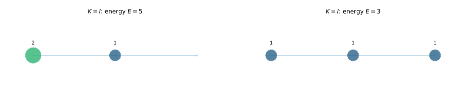
Thus Theorem 8.1, the spectral bound, and the separation estimate are distinct statements. None, by itself, says that strict local descent always solves the global integer minimization problem.
9 Stationary potentials and the mesh-dependent gradient bound
9.1 The coordinate-free graph statement
For a constant-diagonal kernel and an ascent-stationary \(c\), the exact inequality is
This is the natural graph analogue of a gradient condition. On an abstract graph there is no Euclidean vector \(\nabla V_{c}(p)\) until an embedding and a smooth extension have been specified.
9.2 A general symmetric-stencil estimate
Lemma 9.1 (Taylor control at a stationary grid site). Let \(V\) be twice differentiable on the two coordinate segments \(p+se_{j},|s|\le h\), and assume
Then
The right side is necessarily nonnegative whenever these hypotheses are simultaneously satisfied.
Proof. Taylor’s theorem gives points \(\xi _{+}\in (0,h)\) and \(\xi _{-}\in (-h,0)\) with
Combine each lower Taylor bound, using \(|\partial _{jj}V|\le L_{j}\), with the corresponding upper stationarity bound. This yields \(h\partial _{j}V(p)\le h^{2}L_{j}/2-\alpha _{j}\) and \(-h\partial _{j}V(p)\le h^{2}L_{j}/2-\alpha _{j}\). Divide by \(h.\quad \square\)
9.3 The unperturbed torus: retaining the original estimate
Use the period-\(N\) smooth extension
Set \(\omega =2\pi /N\). Direct differentiation gives
Since \(k_{N}\le e^{\beta d},\)
The nearest-neighbor correction is
At a stationary occupied site, (9.1) holds in both coordinate directions. Apply Theorem 9.1 with \(h=1\):
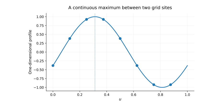
For fixed \(n,d,\beta\), the right side is \(O(N^{-2})\) as \(N\to \infty\), since \(\delta _{N}=O(N^{-2})\). This estimate holds for every positive \(\beta\), not only in the concentration regime.
The order changes when coordinates change
The \(O(N^{-2})\) bound is written in period-\(N\) coordinates, where one move has length one and the kernel contains 2\(\pi /N\). In unit-torus coordinates \(u=z/N\), let \(\widetilde{V}(u)=V_{N}(Nu)\). Then \(\nabla _{u}\widetilde{V}=N\nabla _{z}V_{N}\), so the corresponding bound is \(O(N^{-1})\). This is the same estimate in different units, not a contradiction. For large \(\beta\), the constant also contains \(\beta (1+\beta )e^{\beta d}\); the asymptotic order alone can therefore be numerically misleading.
10 A reproducible experimental atlas
10.1 What the experiments are designed to test
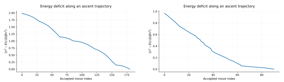
The purpose of the numerical companion is not to estimate a universal “success rate” from a handful of random runs. Each experiment isolates a mathematical issue: a periodic grid inside the geometric theorem, a non-product spherical graph, a branching tree, a sharp tree obstruction, or a repulsive trajectory. The same implementation computes the exact one-particle increment formula throughout. For reproducibility, the selection rule is global steepest improvement, with deterministic lexicographic tie-breaking up to the rounding convention described in Section 11.
| Experiment | \(M\) | \(n\) | \(\beta\) | Moves | Final support |
|---|---|---|---|---|---|
| Torus, ascent | 64 | 48 | \(3\times10^{-4}\) | 180 | 1 |
| Spherical cloud, ascent | 26 | 40 | \(1.864\times10^{-5}\) | 90 | 1 |
| Branching tree, ascent | 15 | 12 | 0.02 | 36 | 1 |
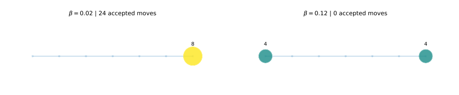
| Path, below threshold | 7 | 8 | 0.02 | 24 | 1 |
| Path, above threshold | 7 | 8 | 0.12 | 0 | 2 |
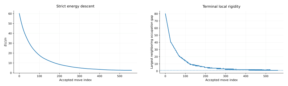
| Torus, descent | 64 | 160 | 22 | 559 | 64 |
| Cycle, spherical kernel | 6 | 6 | 0.01 | 8 | 1 |
| Cycle, distance kernel | 6 | 6 | 0.01 | 0 | 3 |
\(M\) is the number of vertices. “Moves” counts accepted one-particle moves. The cloud’s parameter is rounded in this table; the full value and every initial occupation are recorded in data/manifest.json. The theorem bounds and the numerical stopping tolerance are different quantities.
All energies in the experiments use kernels with unit diagonal. The geometric kernels are \(e^{-\beta a_{xy}}\), and the tree kernels are \(e^{-\beta d_{G}(x,y)}\). Thus a Dirac configuration has energy \(n^{2}\), which makes the normalized energy \(E/n^{2}\) a convenient display quantity. This normalization does not make the different models dynamically identical.
10.2 An irregular spherical graph: no Fourier coordinates required
For the non-product experiment, draw 26 independent Gaussian vectors in \(\mathbb{R}^{3}\) and normalize each to unit length, using random seed 17. Compute the convex hull and retain its 72 edges. The spherical interaction uses the resulting three-dimensional coordinates, not the two-dimensional projection used in the HTML viewer. Distribute 40 particles by a uniform multinomial draw with seed 71. Choose
This choice lies inside the sufficient geometric regime by construction. The theorem guarantees concentration from every initial occupation on this fixed graph; the displayed trajectory is one example, terminating after 90 accepted moves.
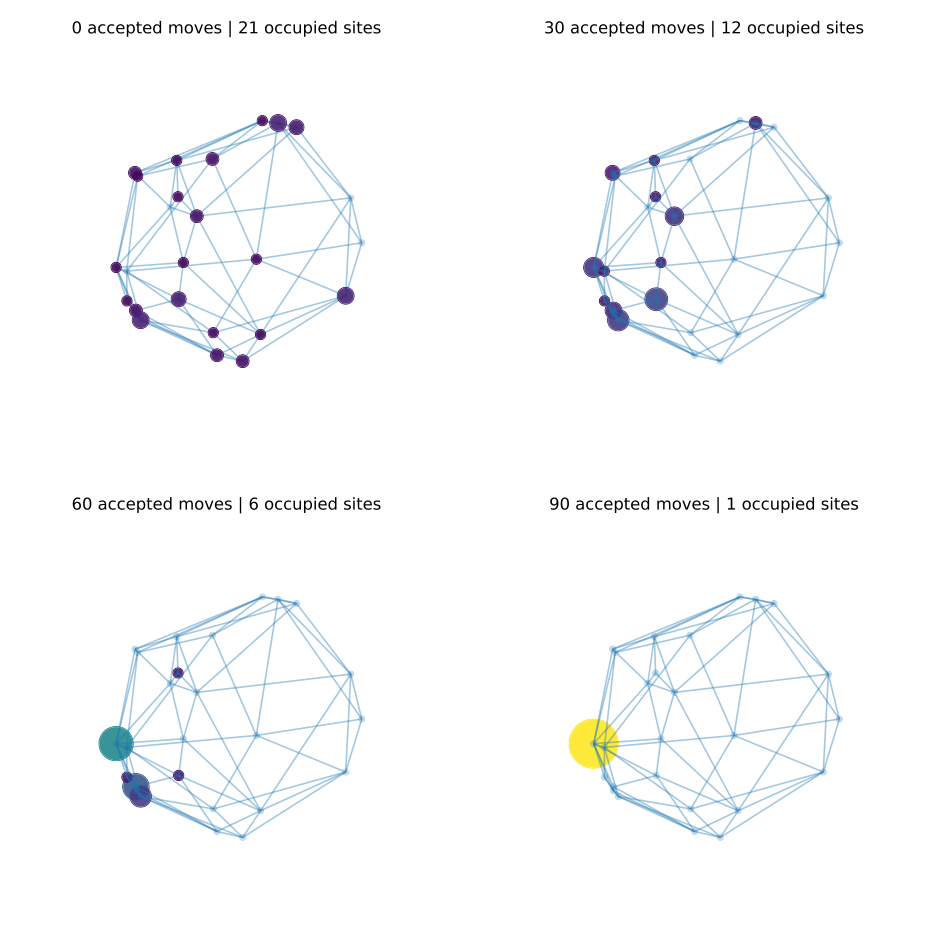
Animation 5. cloud_ascent.mp4. The offline companion gallery.html provides playback and a state-by-state slider.
10.3 Repulsion: large change in occupation, modest local gaps
The descent example starts from three occupied sites of an 8 \(\times 8\) periodic grid, with occupations 80, 40, 40, and takes \(\beta =\) 22. For this graph,
so the sufficient rigidity condition (8.6) applies. The terminal occupation field has 64 occupied sites, each containing two or three particles. Its maximal neighboring imbalance is one, exactly as predicted. This particular near-uniformity is stronger than the neighboring-gap statement alone; it should not be promoted to a general consequence without proof.
10.4 Enumeration on a small state space
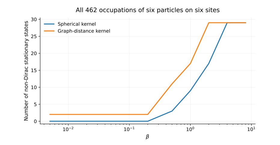
Six particles on six sites have \(\binom{6+6-1}{6-1}=462\) possible occupation fields. We enumerate all of them on \(C_{6}\) at eleven parameter values, and test every legal outgoing move. For the spherical kernel, no non-Dirac stationary state is found at the sampled values up to \(\beta =0.2\); some are found at \(\beta =0.5\)
and above. The sufficient theorem bound in this example is only 1\(/40\). The enumeration therefore illustrates the conservatism of that bound, but it does not identify an exact transition parameter. For the distance kernel, non-Dirac stationary states already occur at the smallest tested parameter. The explicit three-cluster obstruction in (7.4) proves their existence for every positive parameter, independently of this computation.
What has been checked, and what has been proved
The executable verification suite checks 4,057 random evaluations of the exact increment identity, 1,676 non-Dirac spherical configurations in the sufficient regime, and 1,965 non-Dirac tree configurations below the analytical threshold. It also checks the explicit tree obstructions. These tests help detect coding, normalization and sign errors. They are not substitutes for the proofs, and floating-point enumeration is not an interval-arithmetic certificate.
10.5 How to read the animations
The five movies each last ten seconds and are encoded at 24 frames per second. Their duration is a presentation choice, not an algorithmic running time. Particle occupations are linearly interpolated between selected integer states for visual smoothness; these fractional displays are not extra states of the discrete algorithm. The accepted-move counter, energy and support size report the last completed integer state. A moving marker follows the currently displayed transfer where its drawing is unambiguous. The sphere movie rotates the camera, not the underlying vertices.
For exact inspection, use gallery.html: its slider selects integer accepted states, so every displayed occupation has total mass \(n\). All trajectory arrays are embedded in that HTML file; no server, external script or internet connection is required. The torus is drawn as a periodic square grid with boundary stubs. Periodic partners remain neighbors even when their connection is not drawn as a long line across the square. The three-dimensional torus illustration in Section 3 is a
drawing of the graph, whereas the interaction embedding of \(C_{8}\square C_{8}\) is in \(\mathbb{R}^{4}.\)
11 Implementing the algorithm without changing the mathematics
11.1 Why maximizing the potential is not always the right move
For a fixed source \(p\), the accepted destination maximizes
not necessarily \(V_{c}(q)\). Consider the symmetric kernel and occupation
on a graph containing the edges 0\(\sim\)1 and 0\(\sim\)2. For a particle at \(p=0,\)
but the exact increments are
Potential ranking prefers vertex 1, whereas exact-increment ranking prefers vertex 2. On the isotropic nearest-neighbor torus, \(K(p,q)\) is constant over the neighbors of \(p\), so the rankings agree. That special simplification must not be silently carried to an irregular geometric graph.
11.2 Updating a cached potential
Once \(V=Kc\) is known, all legal increments follow from (2.4). After accepting \(p\to q,\)
This is an \(O(M)\) update for a dense stored kernel. Scanning both orientations of all edges costs \(O(|\mathcal{E}|)\), and storing a dense kernel costs \(O(M^{2})\) memory. Thus a cached-potential implementation can perform one global selection and update in \(O(M+|\mathcal{E}|)\) arithmetic operations, after initialization. These are arithmetic-operation counts, not measured wall-clock benchmarks. Periodic convolution offers an alternative \(O(M\operatorname{log} M)\) potential evaluation through the discrete Fourier transform; it is a computational convenience of the torus, not a hypothesis of the geometric concentration theorem.
The supplied reference implementation deliberately evaluates the leave-one-out formula directly. This costs more on a dense graph but makes the mathematical correction transparent and avoids accumulation of cached-update drift. The numerical examples are small enough that clarity is preferable to a specialized high-performance implementation.
11.3 Small parameters and cancellation
When \(\beta\) is small, \(e^{-\beta a_{xy}}\) is close to one, while the useful differences are of size \(\beta\). Compute instead
\(L_{xy}=\operatorname{expm1} (-\beta a_{xy})=e^{-\beta a_{xy}}-1.\)
Since \(K=L+\mathbf1\mathbf1^{\top}\), the two energies differ by the constant \(n^{2}\) on \(\mathcal{C}_{n}\), and their increments agree exactly. The routine expm1 evaluates the small difference directly. In the supplied code, this
shifted representation is used when \(\beta A<1/2\); otherwise the unshifted kernel is used. The displayed energy is always restored to the unit-diagonal normalization.
A tolerance is not part of the exact mathematical dynamics. In floating point, the code accepts an ascent move only when its computed increment exceeds \(\tau =2\times 10^{-12}\), and a descent move only when it is less than \(-\tau\). It records the largest improvement score at termination in terminal_score; a nonpositive value means that the computed outgoing increments all have the correct terminal sign. The manifest also records the tolerance and the tie convention. Near a critical parameter, formal certification would require error bounds or exact arithmetic, not merely a smaller tolerance.
11.4 A complete reproduction route
The source bundle contains the manuscript, vector and raster figures, trajectory arrays, an offline viewer, five movies and the two Python modules that produced them. From the bundle directory, a typical reproduction sequence is
python -m pip install -r code/requirements.txt
python code/reproduce.py --check
python code/reproduce.py --figures
python code/reproduce.py --movie torus_ascent
python code/reproduce.py --movie cloud_ascent
python code/reproduce.py --movie tree_ascent
python code/reproduce.py --movie torus_descent
python code/reproduce.py --movie cycle_ascent
python code/build_gallery.py
latexmk -pdf -interaction=nonstopmode graph_particle_notes.tex
Movie encoding additionally requires ffmpeg on the executable search path. The figure exports are PDF and SVG, with PNG previews. Compilation of the supplied manuscript requires no Python execution: the ready-made PDF figures are already included. A separate README.md gives the tested environment and the precise layout of the bundle.
12 What the generalization teaches us
The original torus model is not merely an isolated Fourier calculation. Its unperturbed interaction is an exponential Gram kernel, and its nearest-neighbor graph is the skeleton of an inscribed product polytope. That geometric compatibility is enough to rule out all non-Dirac local traps at small positive parameter. The first Fourier modes are useful coordinates for the torus barycenter, but the barycenter argument survives when no translation symmetry or Fourier diagonalization remains.
The tree theorem expresses a different mechanism. A leaf of the occupied subtree can move toward every other occupied vertex simultaneously. Concentration follows when this collective gain dominates the loss of interaction with the particles left behind at that leaf. Two clusters at a diameter’s endpoints balance that competition exactly at a computable threshold. On a cycle, competing directions can destroy this mechanism. These are structural facts about the graph–kernel pair, not consequences of attraction alone.
The AI connection should be read at the same level of precision. Self-attention gives a natural motivation for exponential similarity weights and for asking when interacting representations lose diversity. The present results make a related question completely explicit in a finite dictionary with constrained moves. They do not assert that a trained attention block optimizes this energy, that a particular Transformer will collapse, or that repulsion alone improves task performance.
The contribution is a mathematical testbed in which global energy preferences, local accessibility, the role of discretization and the failure of naive convergence arguments can all be separated.
Several directions are natural and are not settled by these notes. One is to characterize graph– kernel pairs satisfying the abstract strict-local-maximum criterion of Section 4. Another is to sharpen the sufficient spherical threshold, whose uniform Taylor bound can be conservative. A third is to understand terminal descent states beyond neighboring rigidity, distinguishing local stationary states from global integer minimizers. Finally, varying particle number and refining a graph simultaneously changes the quantitative small-parameter window; the fixed-\(n\), fixed-graph theorem must not be interpreted as a uniform continuum-limit result.
Problems for further study
Exercise 12.1 (A complete graph with identical off-diagonal weights). Take \(K_{xx}=\kappa\) and \(K_{xy}=b<\kappa\) for \(x\ne y\), with 0 \(\le b\). Prove
Deduce that ascent terminates at a Dirac state, and that descent terminates at an integer minimizer whose occupations differ by at most one. Explain precisely which conclusion fails if the move graph is a path.
Exercise 12.2 (A weighted product embedding). Replace (5.1) by
where \(r_{j}>\) 0 and \(N_{j}\ge\)3. Show that
Write explicit concentration and global-steepest move bounds. Compare what happens when one coordinate radius tends to zero with what happens when one cycle is refined.
Exercise 12.3 (From a counterexample to a mechanism). On \(C_{6}\) with the distance kernel, compute the two changes in interaction created by moving one particle away from an occupied even vertex in (7.3): the loss to its companion and the opposing changes to the two other clusters. Explain the factor 2\(r(1-r)\) in (7.4), and why connectedness does not prevent the trap.
A The smooth-profile proof on the torus, in full
This appendix preserves the analytical route that is useful when one wishes to inspect the perturbed one-dimensional potentials themselves. It is not needed for the stronger geometric robustness theorem, which requires only a uniform bound on the symmetric perturbation. Keeping the two arguments separate clarifies which hypotheses belong to which conclusion.
A.1 Stability of nondegenerate critical points
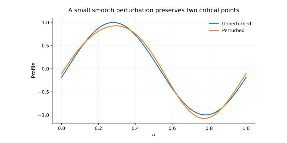
Proposition A.1 (A complete perturbation lemma). Let \(g_{0}\in C^{2}(\mathbb{T}^{d};\mathbb{R})\) have finitely many critical points, all nondegenerate. Suppose \(r_{\eta}\in C^{2}(\mathbb{T}^{d};\mathbb{R})\) and \(\|r_{\eta}\|_{C^2}\to 0\) as \(\eta \to 0\). Then, for sufficiently small \(\eta ,g_{\eta}=g_{0}+r_{\eta}\) has exactly the same number of critical points as \(g_{0}\). They can be labeled \(z_{i}(\eta )\) so that \(z_{i}(\eta )\to z_{i}\), and corresponding critical points have the same Morse index.
Proof. Write Crit\((g_{0})=\{z_{1},...,z_{s}\}\). Choose mutually disjoint coordinate neighborhoods around these points. Within each neighborhood, use a Euclidean lift and choose a closed ball \(\overline{B}_{\rho _{i}}(z_{i})\) contained in that coordinate chart, with no other critical point of \(g_{0}\) in it. Set \(H_{i}=D^{2}g_{0}(z_{i})\); it is invertible. By continuity of the Hessian, the balls can be chosen so small that
Because there are finitely many \(i\) and \(r_{\eta}\to\)0 in \(C^{2}\), one common smallness threshold ensures
Define
Equations (A.1)–(A.2) imply \(\|D\Phi _{i,\eta}\|\le 1/2\) throughout the ball. The mean value inequality therefore shows that \(\Phi _{i,\eta}\) is a contraction there. Moreover, since \(Dg_{0}(z_{i})=0,\)
Thus the map sends the closed ball into itself. The contraction mapping theorem gives a unique fixed point \(z_{i}(\eta )\) in that ball. Because \(H_{i}\) is invertible, its fixed-point equation is equivalent to \(Dg_{\eta}=\) 0. The same estimate with \(x=z_{i}(\eta )\) gives
It remains to rule out other critical points. Let \(Q\) be the complement of the union of the open balls. It is compact and has no critical point of \(g_{0}\), so
After shrinking the perturbation threshold so that \(\|Dr_{\eta}\|_{\infty}<m_{0}/2\), one has \(\|Dg_{\eta}(x)\|\ge m_{0}/2\) on \(Q\). Hence the critical points already constructed are the only ones.
Finally,
Let \(\gamma _{i}\) be the smallest absolute eigenvalue of \(H_{i}\), which is positive. Once the last matrix difference is smaller than \(\gamma _{i}/2\), the variational characterization of eigenvalues of symmetric matrices shows that no eigenvalue changes sign. The perturbed critical point is therefore nondegenerate and has the same number of negative eigenvalues, namely the same Morse index. Finitely many critical points allow one final common smallness threshold.\(\square\)
A.2 Uniformity over discrete particle configurations
Use unit-torus coordinates and an even \(C^{2}\), one-periodic function \(f_{j}\) in each coordinate. For a labeled configuration \(z=(z_{1},...,z_{n})\in (\mathbb{T}_{N}^{d})^{n}\), write
where \(A_{j}(z)=\sum _{i}e^{-2\pi iz_{i,j}}=|A_{j}(z)|e^{-2\pi i\theta _{j}(z)}\). If \(A_{j}(z)\ne 0\), the cosine term has exactly two critical points, one maximum and one minimum, with second derivatives \(-4\pi ^{2}|A_{j}|\) and 4\(\pi ^{2}|A_{j}|.\)
Lemma A.2 (Uniform two-critical-point structure). For fixed \(n,N,d\) and \(f_{1},...,f_{d}\), there is an \(\eta _{\ast}>0\) such that whenever \(|\eta _{j}|<\eta _{\ast}\) and \(A_{j}(z)\ne 0\), the function \(\phi _{j}^{z}\) has exactly one nondegenerate maximum and one nondegenerate minimum on the circle.
Proof. There are only finitely many labeled grid configurations. Consequently
The set in this minimum is nonempty, since a Dirac configuration has \(|A_{j}|=n\). Each unperturbed profile satisfies the hypotheses of Theorem A.1, and its perturbation has the bound
Apply that proposition to every nonzero-mode profile and take the minimum of the finitely many resulting thresholds, and then the minimum over \(j\). This proves the required uniform statement.
The positive number \(m_{j}\) also explicitly records why nondegeneracy cannot degenerate while \(n,N\) remain fixed. No uniform lower bound as \(n\) or \(N\) varies has been asserted.\(\square\)
A.3 Sampling a unimodal function on a cycle
A non-strict discrete local maximum is a vertex whose value is at least that of both cycle neighbors. A strict one requires both inequalities to be strict.
Lemma A.3 (The adjacent-maximum alternative). Let \(f\in C^{1}(\mathbb{T})\) have exactly one maximum and one minimum, and be strictly monotone on each of the two arcs between them. Sample it at \(N\ge 3\) equally spaced sites. The sampled non-strict local maxima consist of either one site, or two neighboring sites having equal values. In particular, there is at most one strict discrete local maximum.
Proof. If the continuous maximum is a sampled site, every other sampled site can move one step toward it along an arc of strict increase, except possibly across an interval containing the minimum. At such an interval, the neighbor on the other side of the candidate site lies on a strictly increasing path toward the maximum. Thus the maximum site is the only sampled local maximum.
More explicitly, when the maximum lies strictly between two consecutive sampled sites, call them \(u\) and \(v\). Remove the open grid interval \((u,v)\) containing that maximum. On the remaining oriented arc from \(v\) to \(u\), the function first decreases toward its sole minimum and then increases, if that minimum belongs to the remaining arc. Every sampled site other than the endpoints therefore has a strictly larger neighbor: this is immediate on either monotone side, and holds for each of the at most two sampled sites bracketing the minimum by taking its other neighbor. If the minimum instead lies in the removed interval, the function is strictly monotone on the entire remaining arc, with the same conclusion for interior sampled sites. Hence all sampled local maxima are among \(u,v.\)
If \(f(u)>f(v)\), then \(v\) cannot be a local maximum because it is adjacent to \(u\); if \(f(v)>f(u)\) the reverse holds. At least one sampled local maximum exists by finiteness, so there is exactly one in these cases. If \(f(u)=f(v)\), the strict monotonicity away from the continuous extrema shows that the other neighbor of each endpoint has smaller value; equivalently, neither endpoint can fail to be a maximum without an interior maximum on the remaining arc. Thus both are non-strict local maxima. They are adjacent and neither is strict.\(\square\)
The continuous profiles from Theorem A.2 meet the monotonicity hypothesis: their derivative is nonzero off the two critical points, so its sign is constant on each complementary arc. By (A.3), a grid point is a non-strict local maximum of \(S_{z}\) if and only if each coordinate is a non-strict sampled maximum of the corresponding profile. Hence
and any two points in an \(M_{j}^{z}\) with cardinality two are neighbors and have equal profile values. This is the precise product fact needed by the original torus argument.
A.4 The stationary gap for a general perturbed profile
Let \(\sigma\) be symmetric, translation invariant, with constant diagonal \(\sigma _{\ast}\), and define
Assume \(L:=\max_{x,y}|\sigma(x,y)|<\infty\). For all \(|s|\le L\), Taylor’s theorem gives
The lower bound is the tangent-line inequality for the exponential, valid also for negative \(s\). The leave-one-out computation used in Theorem 4.2 consequently yields
If \(c\) is ascent-stationary, division by 2\(\beta\) gives
Thus a positive diagonal-to-edge gap forces every occupied stationary site to be a strict sampled maximum for sufficiently small positive \(\beta\). The explicit remainder makes clear that the statement is uniform over configurations, not merely valid one configuration at a time.
For the separable perturbed torus profile, \(\sigma _{\ast}-\sigma (p,q)\) tends uniformly over edges to \(\delta _{N}>0\) as all \(\eta _{j}\to 0\). Choose the perturbation size so that this gap is at least 3\(\delta _{N}/4\) and so that \(L\) has a common finite bound. Next choose \(\beta _{\ast}>0\) so that the last term in (A.7) is at most \(\delta _{N}/4\) for 0 \(<\beta <\beta _{\ast}\). Then
A.5 Closing the original perturbative concentration proof
Theorem A.4 (The smooth-profile route to torus concentration). For fixed \(n\ge 2,N\ge 3,d\ge 1\) and even functions \(f_{j}\in C^{2}(\mathbb{T})\), there exist \(\eta _{\ast},\beta _{\ast}>0\) such that \(|\eta _{j}|<\eta _{\ast}\) and 0 \(<\beta <\beta _{\ast}\) force every ascent-stationary configuration for the perturbed torus kernel to be a Dirac state. Every complete ascent implementation therefore terminates at a Dirac state from every initial occupation.
Proof. Shrink \(\eta _{\ast}\) as necessary so that Theorem A.2 and (A.8) apply, and also so that
Let \(c\) be stationary. We first prove \(A_{j}(c)\ne 0\) for all \(j\). If \(A_{j}(c)=0\), the unperturbed cosine contribution in coordinate \(j\) vanishes identically. Take an occupied site \(p\) and its neighbor \(q\) in the \(j\) th coordinate direction. All other coordinate contributions cancel, giving
contrary to (A.8). Thus every coordinate mode is nonzero at a stationary state. This is a terminal-state argument; it does not assume, or need to prove, persistence of nonzero modes along the trajectory.
The uniform profile lemma and Theorem A.3 now yield the product structure (A.5). Every occupied site is a strict sampled local maximum of \(S_{c}^{\sigma}\) by (A.8). If some \(M_{j}^{c}\) had two elements, changing that coordinate of any occupied site to the other element would be a legal neighbor move with exactly the same value of \(S_{c}^{\sigma}\), contradicting the strict gap. Therefore each \(M_{j}^{c}\) is a singleton, so their product is a singleton and the support of \(c\) is contained in that one point. Its total mass is \(n\), hence \(c=n\delta _{x}\). Finite termination and completeness finish the argument.\(\square\)
The geometric proof supplies explicit constants and permits arbitrary small symmetric perturbations, rather than only smooth separable ones. The profile proof supplies additional information about the continuous one-dimensional critical points. Neither should be used to claim a result it does not establish: smooth critical-point stability needs \(C^{2}\) control, whereas discrete concentration in the geometric setting does not.
References
[1] A. Vaswani, N. Shazeer, N. Parmar, J. Uszkoreit, L. Jones, A. N. Gomez, Ł. Kaiser and I. Polosukhin. Attention Is All You Need. Advances in Neural Information Processing Systems 30 (2017). arXiv:1706.03762.
[2] B. Geshkovski, C. Letrouit, Y. Polyanskiy and P. Rigollet. The emergence of clusters in self-attention dynamics. Preprint (2023). arXiv:2305.05465.
[3] B. Geshkovski, C. Letrouit, Y. Polyanskiy and P. Rigollet. A mathematical perspective on Transformers. Preprint (2023). arXiv:2312.10794.
[4] B. Geshkovski, H. Koubbi, Y. Polyanskiy and P. Rigollet. Dynamic metastability in the self- attention model. Preprint, version 1 (2024). arXiv:2410.06833.
[5] Y. Dong, J.-B. Cordonnier and A. Loukas. Attention is not all you need: pure attention loses rank doubly exponentially with depth. Proceedings of the 38th International Conference on Machine Learning, PMLR 139 (2021), 2793–2803. Publisher’s page.
[6] H. Ramsauer et al. Hopfield Networks is All You Need. Preprint (2020). arXiv:2008.02217.
[7] P. Veličković, G. Cucurull, A. Casanova, A. Romero, P. Liò and Y. Bengio. Graph Attention Networks. International Conference on Learning Representations (2018). arXiv:1710.10903.
[8] G. M. Ziegler. Lectures on Polytopes. Graduate Texts in Mathematics 152, Springer, 1995.
doi:10.1007/978-1-4613-8431-1.
[9] A. Padrol and G. M. Ziegler. Six topics on inscribable polytopes. Preprint (2015). arXiv:1511.03458.